ML Modeling of Reactivity Descriptors of Metal Clusters toward N₂ Activation

GitHub Repo: https://github.com/kunlun-wu/mlms-final/tree/main/nic-raffaele-kunlun-wu

Overview

Inspired by L. Mou, et al. Unveiling Universal Reactivity Descriptors of Metal Clusters toward Dinitrogen Activation: A Machine Learning Protocol with Three-Level Feature Extraction. ACS Catalysis 2025 15 (8), 6618-6

Dataset obtained from GitHub Repo provided by original authors.

1. The Problem

• How do we predict a material’s effectiveness in use as a catalyst for N₂ activation towards ammonia?

2. Significance

• N 𝄘 N bonds are one of the strongest in chemistry, activation depends on subtle electronic and geometric effects across different metals and ligands.

3. Models Implemented

• Supervised learning regression models:
  • Support Vector Regression (SVR) with RBF and polynomial kernels
  • Random Forest Regression (RFR) with Recursive Feature Elimination (RFE) and SelectKBest feature selection
  • Multilayer Perceptron (MLP) models—both from scikit-learn and a self-compiled architecture

4. Dataset

• 216 total cluster-N₂ rxn measurements:
  • 159 homonuclear clusters
  • 57 heteronuclear clusters

5. Features and Labels

• Three level feature extraction yielding 24 features:
  • Site level: maximum/minimum natural charge
  • Local environment: average spin density, valence d-occupancy, total charge, etc.
  • Cluster level: polarizability, dipole, electronegativity, ionization energies, etc.
• Labels are the The logarithmic rate constant, lg(k₁), ranging roughly from –15 to –9

Understanding the Data

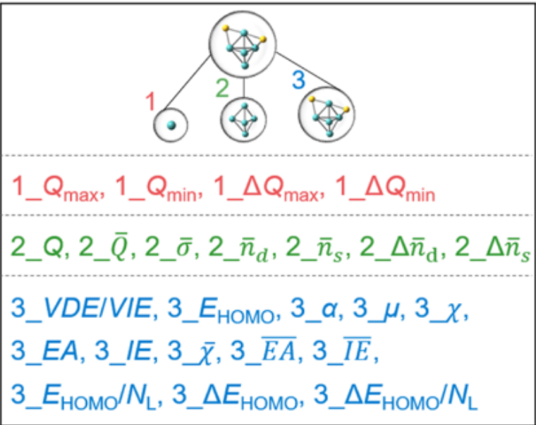
• All 24 candidate features derived from the three-level feature extraction, illustrated using the structure of Mo₅S₂⁻. Figure adapted from original paper.
• Site level features are marked with 1, local environment level features are marked with 2, and cluster level features are marked with 3.
• In the excel datasheet, the feature descriptors starts from Column 3 of the data until the end. Column 2 is the target lg(k₁) and Column 1 are the names for individual clusters (Rows are individual clusters).

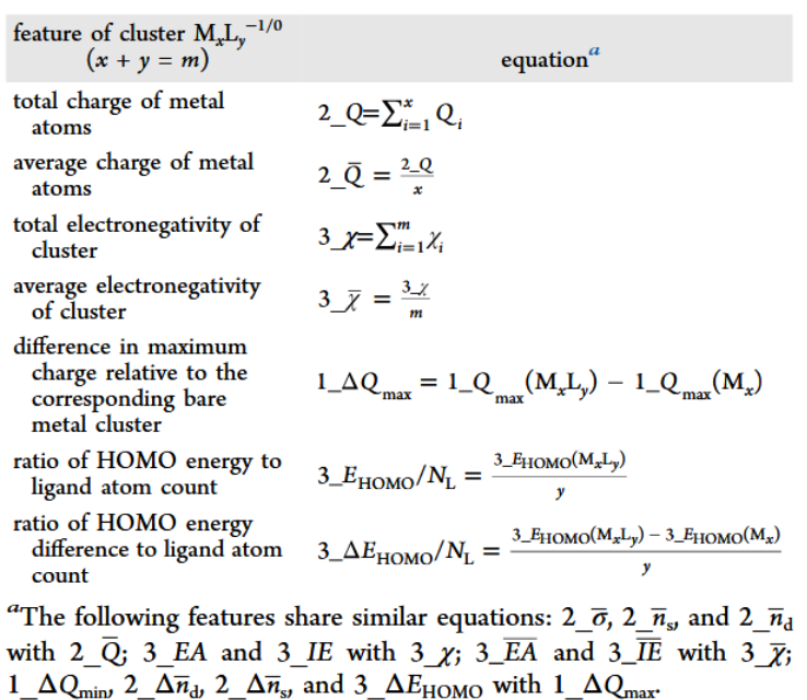
• Equations for computing some representative features, table adapted from original paper.

The authors found that none of the individual descriptors map to lg(k₁) linearly. Some features like average spin density show threshold‑type behavior rather than a constant slope. Others like ΔE_HOMO/N_L interact multiplicatively with site‑level charges, producing curved or segmented trends. To verify we plotted each feature against the label (code can be found in feature-label-relationship.py):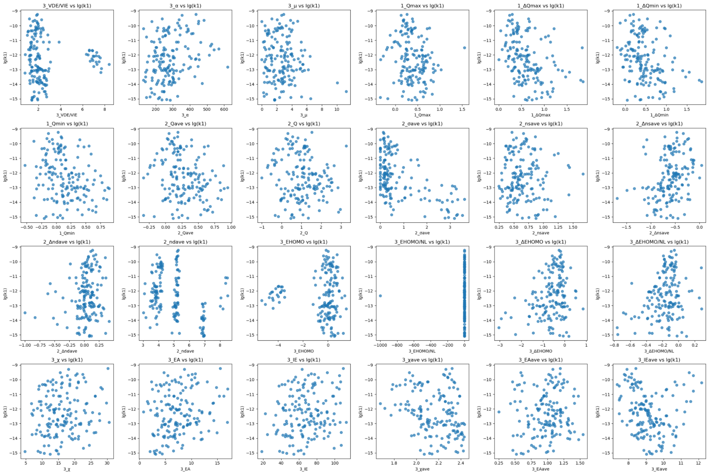

Feature Engineering

• Proposed Models: based on the nonlinearity, it is best to use models that capture complex relationships
  • SVR: Offers alternative paradigms for smooth function approximation and uncertainty estimation.
  • RFR: Interpretable, handles mixed feature types, robust to medium-small datasets without scaling.
  • MLP from sklearn: Captures high-order interactions and non-linearities, especially combined with feature interactions. This model from sklearn gives easily adjustable hyperparameters but less customizability.
  • MLP self-compiled from tensorflow: This self-compiled model gives more freedom in customizing the layers than the preconfigured one from sklearn.
• Feature Selection and Scaling:
  • Selectors:
    • RFE: recursively removes least important features based on model weights. It optimizes to each model individually. However, it requires the model being evaluated to expose .feature_importances or .coeff_ attributes to work, so in our case it only worked with RFR.
    • SelectKBest: computes a univariate score for each feature against the target. So it is model-agnostic. f_regression performs an ANOVA F‑test by fitting a simple linear model to each feature individually and measuring how much of the variance in y it explains. It is also pipeline-friendly.
  • Scalers: not needed for RFR but important for SVR and MLP as they are sensitive to feature magnitudes.
    • StandardScaler: Centers features to have mean 0 and variance 1.
    • MinMaxScaler: Scales features to a given range, usually [0, 1].
    • RobustScaler: Centers and scales features using statistics that are robust to outliers (median and IQR).

Developing the Models

We built a framework (main.py) for model training, where run_everything implements an outer KFold loop to evaluate model generalization: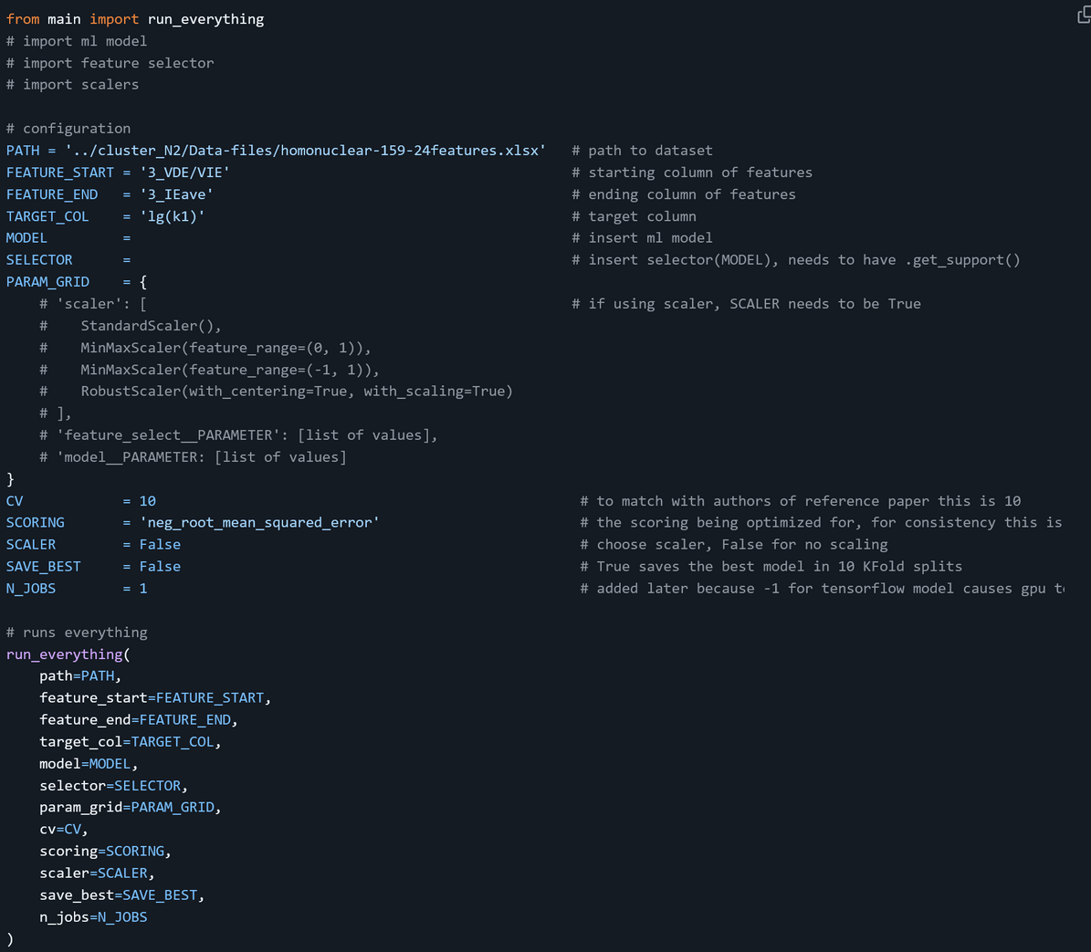

1. Load the Excel dataset and extract feature and target columns.
2. Optionally scale the entire feature set if a scaler is provided.
3. Initialize performance containers and best‐model trackers.
4. For each of the cv folds: a. Split X_full/y_full into X_train/X_test and y_train/y_test. b. Call gridsearch_featureselect on X_train/y_train to fit an inner‐CV pipeline. c. Use evaluate_model to predict on both train and test splits and compute Pearson r and RMSE. d. Store fold metrics, aggregate predictions, and update the best‐model if this fold’s test r is higher.
5. After all folds, print the average of train/test r and RMSE.
6. Report the best fold’s metrics and selected features, save the best model if requested.
7. Produce a combined parity plot overlaying all train and test predictions.

run_everything encapsulates data loading, optional scaling, nested CV tuning, evaluation, and visualization in a single entry point without needing to rewrite functionalities required across models.

The pipeline is dynamically constructed in gridsearch_featureselect: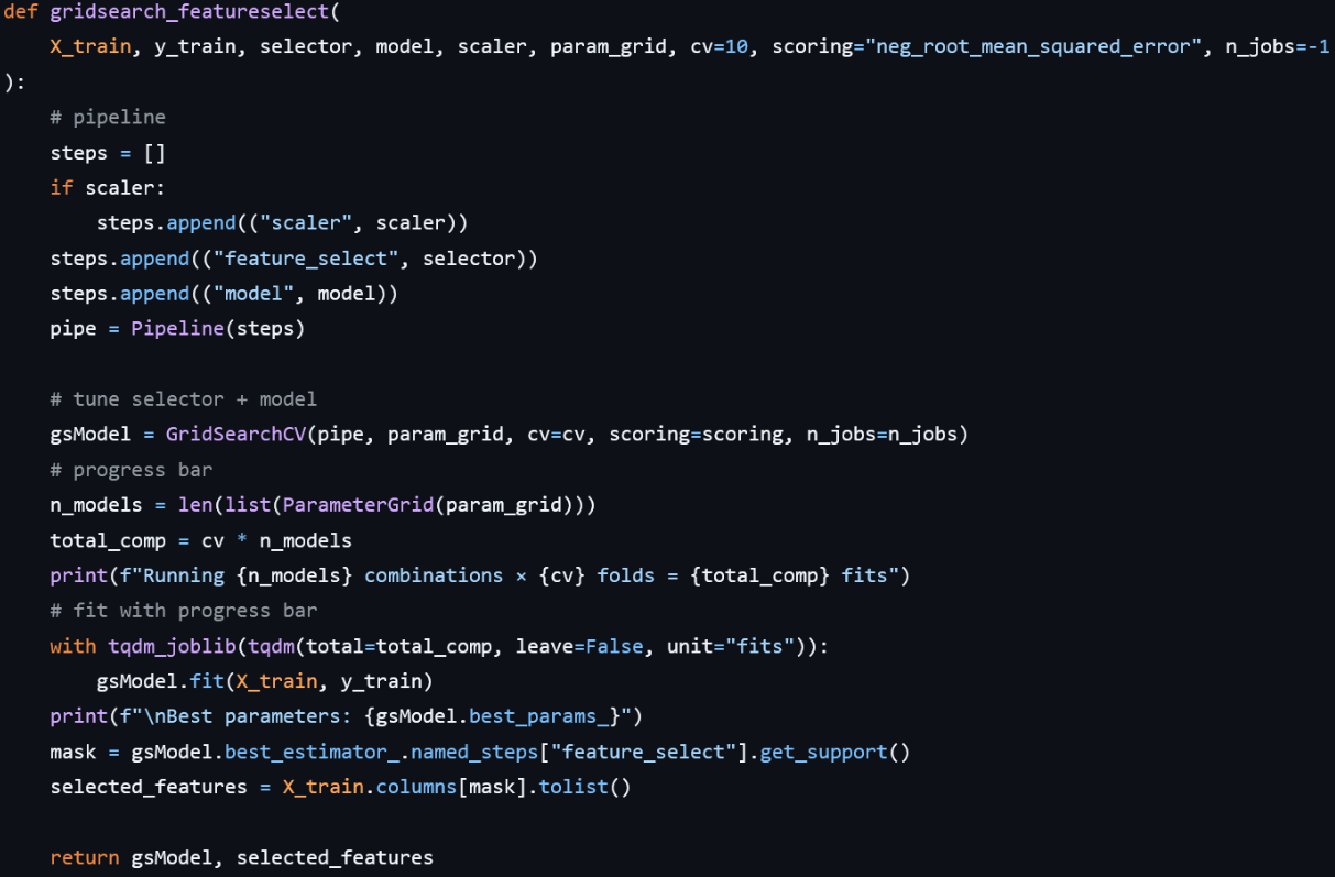

1. If a scaler is provided, it adds (‘scaler’, scaler) as the first step, ensuring each fold is scaled separately.
2. It then adds (‘feature_select’, selector) to remove irrelevant features.
3. Finally, it appends (‘model’, model) for the regression algorithm.

This pipeline is passed to GridSearchCV, which iterates over all combinations of hyperparameters defined in param_grid, performing cross-validation for each. A tqdm‐wrapped context shows real‐time progress of total fits (n_models × cv). Once fitting completes, the function prints the best parameters, pulls the support mask from the selector step of the best estimator to identify the chosen features, and returns both the GridSearchCV object and the selected feature names.

Since the results from sklearn MLP was not satisfying, we also self-compiled a keras NN that is compatible with our framework. We can plug it straight into our Pipeline and GridSearchCV. In __init__ it captures hyperparameters—three hidden‐layer sizes, dropout rate, L2 regularization strength (alpha), learning rate, training epochs, batch size, early‐stopping patience, and a random seed. The _build_model method clears any existing Keras session, then constructs a feed‑forward network:

- Input layer matching input_dim
- Dense(units_1) + ReLU + L2
- Dropout(dropout_rate)
- Dense(units_2) + ReLU + L2
- Dropout(dropout_rate)
- Dense(units_3) + ReLU + L2
- Output Dense(1) (linear)
- Compiled with Adam (MSE loss).

The fit method optionally seeds TF, builds the model, and fits it on (X, y) with a 10% validation split and EarlyStopping(monitor='val_loss'), restoring the best weights. After training it clears the session to avoid memory leaks. The predict method returns a flat 1‑D array of predictions, and score computes the Pearson r between y and y_pred (so we can optimize correlation directly in GridSearchCV).

Results and Evaluations

To make sense of how our approach is working, the most effective way is to compare against the authors’ approach. The authors’ code can be found here. Their reported model performance was based on their fold6, which was their best performing split.

To accurately measure their generalization performance, we performed training and testing of the RFR models using their own code for all the folds with slight modifications to keep track of the average scores and produced a comprehensive parity plot.

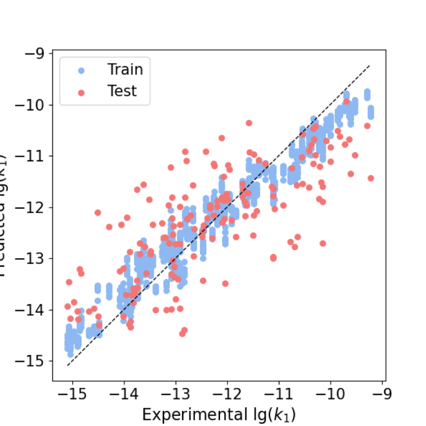
Best train R: 0.98, Best test R: 0.90
Best train RMSE: 0.39, Best test RMSE: 0.50

Average train R: 0.98, Average test R:0.76
Average train RMSE: 0.37, Average test RMSE: 0.97

Our results are shown below:

1. SVR with RBF Kernel + StandardScaler + SelectKBest

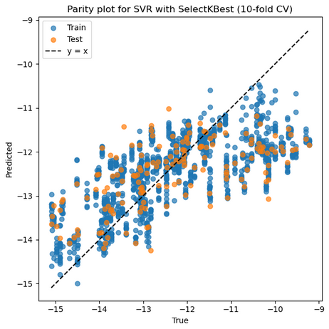
Mean Train r: 0.698, Mean Test r: 0.625
Mean Train RMSE: 1.085, Mean Test RMSE: 1.179

Best parameters: {'feature_select__k': 9, 'model__C': 1, 'model__degree': 2, 'model__epsilon': 0.01, 'model__gamma': 0.01, 'model__kernel': 'rbf', 'model__shrinking': True, 'model__tol': 0.01, 'scaler': RobustScaler()}

Selected features on best fold: ['3_α', '1_ΔQmax', '1_ΔQmin', '1_Qmin', '2_σave', '2_Δnsave', '2_ndave', '3_ΔEHOMO', '3_χave']

Best Train r: 0.663 Best Test r: 0.805
Best Train RMSE: 1.109 Best Test RMSE: 1.377

2. SVR with Polynomial Kernel + StandardScaler + SelectKBest

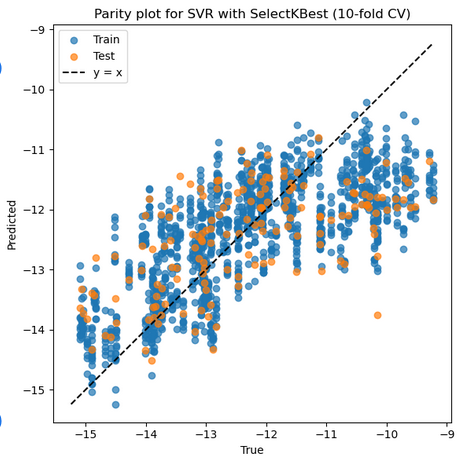
Mean Train r: 0.719, Mean Test r: 0.626
Mean Train RMSE: 1.040, Mean Test RMSE: 1.172

Best parameters: {'feature_select__k': 8, 'model__C': 10, 'model__degree': 2, 'model__epsilon': 0.01, 'model__gamma': 0.01, 'model__kernel': 'rbf', 'model__shrinking': True, 'model__tol': 0.01, 'scaler': StandardScaler()}

Selected features on best fold: ['1_ΔQmax', '1_ΔQmin', '2_σave', '2_Δnsave', '2_ndave', '3_ΔEHOMO', '3_ΔEHOMO/NL', '3_χave'] 

Best Train r: 0.718 Best Test r: 0.822
Best Train RMSE: 1.063 Best Test RMSE: 0.954

3. RFR + RFE + No Scaler

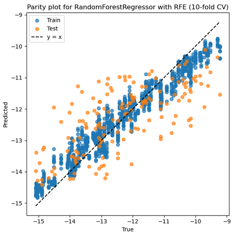
Mean Train r: 0.972, Mean Test r: 0.703
Mean Train RMSE: 0.397, Mean Test RMSE: 1.044

Best parameters: {'feature_select__n_features_to_select': 9, 'model__max_depth': None, 'model__min_samples_leaf': 1, 'model__n_estimators': 200}

Selected features on best fold: ['1_ΔQmax', '1_Qmin', '2_σave', '2_ndave', '3_ΔEHOMO', '3_ΔEHOMO/NL', '3_IE', '3_χave', '3_IEave']

Best Train r: 0.975 Best Test r: 0.904
Best Train RMSE: 0.380 Best Test RMSE: 0.920

4. RFR + SelectKBest + No Scaler

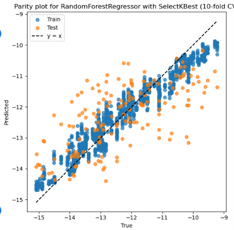
Mean Train r: 0.971, Mean Test r: 0.671
Mean Train RMSE: 0.406, Mean Test RMSE: 1.081

Best parameters: {'feature_select__k': 9, 'model__max_depth': 10, 'model__min_samples_leaf': 1, 'model__n_estimators': 200}

Selected features on best fold: ['3_α', '1_ΔQmax', '1_ΔQmin', '1_Qmin', '2_σave', '2_Δnsave', '2_ndave', '3_ΔEHOMO', '3_χave']

Best Train r: 0.972 Best Test r: 0.907
Best Train RMSE: 0.405 Best Test RMSE: 0.946

5. MLP from sklearn + StandardScaler + SelectKBest

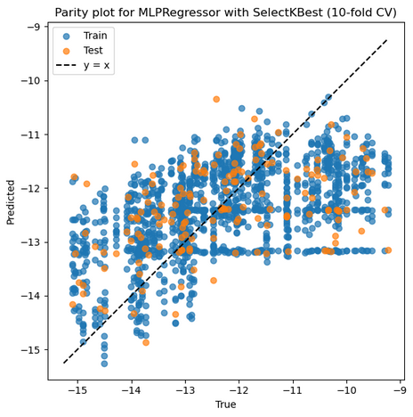
Mean Train r: 0.546, Mean Test r: 0.458
Mean Train RMSE: 1.248, Mean Test RMSE: 1.314

Best parameters: {'feature_select__k': 8, 'model__activation': 'relu', 'model__alpha': 0.01, 'model__hidden_layer_sizes': (100, 50, 25), 'model__learning_rate_init': 0.01, 'model__solver': 'sgd', 'model__validation_fraction': 0.2, 'scaler': MinMaxScaler()}

Selected features on best fold: ['1_ΔQmax', '1_ΔQmin', '2_σave', '2_Δnsave', '2_ndave', '3_ΔEHOMO', '3_ΔEHOMO/NL', '3_χave']

Best Train r: 0.659 Best Test r: 0.769
Best Train RMSE: 1.113 Best Test RMSE: 0.894

6. MLP self-compiled + StandardScaler + SelectKBest

• The self-compiled MLP would take days to run, due to time constraints and other works we have not completed the training. The model training file KerasRegressor.py works though.

Comparison and Analysis

Our RFR model performed the best, RFR natively captures non‑linear interactions and is robust to mixed feature types without requiring strict scaling. Its ensemble averaging reduces variance on a small (~159‑sample) dataset, and recursive feature elimination (RFE) embedded within RFR reliably selected the most predictive 8–9 features per fold, which helped generalization. The feature selector did not impact the results much, we wonder if using pairwise would bring more dominant performance differences

Our SVR performed second best, it is sensitive to hyperparameters and to feature scaling—small mis‑tuning on a modest dataset can lead to under‑ or over‑fitting. Even with careful grid search, SVR struggled to match RFR’s flexibility on high‑order interactions unless enriched with tailored kernels or additional engineered features. The relatively high average RMSE indicates that the decision boundary imposed by the kernel couldn’t fully capture the complex, multi‑level descriptor relationships in this dataset without extensive kernel engineering. The 2 degree poly kernel performed better than rbf kernel, this might be attributed to that it more directly captures the multiplicative interactions that are intrinsic to descriptors.

Our MLP from sklearn performed the worst, this might be attributed to neural networks typically requiring larger datasets to realize their capacity for modelling complex non‑linear mappings. Early stopping and dropout helped avoid over‑fitting, but the net likely under‑fit due to limited epochs and conservative regularization is reflected in low train r (≈ 0.55). The reference paper’s DNN achieved superior results by training on an expanded set of 12,561 pairwise interaction features, which both increased effective sample size and exposed richer structure to the network.

Overall, RFR is the clear winner on this small, feature‑rich dataset due to its robustness and implicit handling of non‑linearities. SVR can be competitive if more expressive kernels or feature interactions are incorporated, but it is tricky in practice. MLPs require substantially more data (or engineered features) to outperform tree‑based methods.

Our RandomForestRegression with RFE and 10 fold cross validation had an average r of 0.703, which is comparable to the referenced RFR as duplicated above with an average r of 0.76.

This difference in label prediction evaluation is likely attributed to the referenced article more rigorous feature extraction. Similar to our approach, the reference evaluated importance using recursive feature elimination embedded in a RFR model. Unlike our feature selection, their features were selected from the highest 10-fold cross validation score after they repeated the RFE pipeline 100 times. Each important feature from each iteration was given a score of 1 if important and all 8 of their features scored 100 points. This difference in feature selection likely accounts for a fair amount of error within our models. Our RFR model-based feature selection, although convenient and quick, likely overfits and outputs features that do not generalize the data as those noted in this reference.

Moreover, thorough SHAP analysis and the strong intuition of the authors helped to guide this original feature selection and their pairwise learning strategy. They were able to strongly argue for each feature selected, correlating to energy states and other intrinsic molecular features on the impact electron transferability to N2. Given more time to research their preliminary DFT calculations and fully understand each feature for how they impact the electronic structure of the metal cluster, we could replicate a stronger feature evaluation.

Our RFR model performed similarly to the references before they enhanced model robustness by creating interaction features using pairwise products aiming to encompass synergistic effects of the original features. This additional pairwise learning that the authors added to the model dramatically improved their RFR performance.Including pairwise interactions is extremely useful and common in atomistic simulations and modeling as it provides some interpretability of unique and underexplored atomic interactions. The authors also noted that expanding their dataset as they trained models on a wider array of original and “enhanced” features aided in model generalization and transferability to heteronuclear structures.In future models and projects, we would encompass a similar pairwise learning method in our study.

Comparing the model that is our project’s best and the reference’s preliminary models trained without an additional 120 enhanced features, we see that our RMSE and r values for the test datasets are comparable, especially when considering the differences in our feature selection and overall workflow. Our other models, SVR and MLP neural net, did not perform as strongly as RFR, as also demonstrated in this article. We attempted to build a self-compiled neural net to compare to the reference’s final DNN model, yet it would take several days to run which is not within the timeline of the project. However, for future works we certainly note the advantages of using a neural net, as also demonstrated in the article. Their DNN was also trained on a much larger dataset as their pairwise learning strategy expanded to 12,561 cluster pairs, helping to reduce error in reaction rate predictions by better interpreting sensitivity to features after incorporating an additional 105 interaction features. Their feature importance analysis on the DNN also outputs several new and highly important interaction features that were not included in our training data set.

Conclusions

Our project aimed to predict the reaction rate of homonuclear metal clusters towards nitrogen activation. The current Haber Bosch process was developed by synthesizing and kinetically testing roughly 2500 catalysts around 6500 times before selecting Fe on gamma alumina as a sufficient catalyst. Machine learning, coupled with DFT calculations, now allows us to predict the reactivity of heterogeneous catalysts, dramatically decreasing the experimental work needed to find an ideal catalyst. In this approach, machine learning is used to predict metal cluster reactivity for heterogeneous catalysts capable of ammonia production. Electrocatalysis provides a promising way to circumvent the high pressure, energy usage, and CO2 output currently needed for the Haber Bosch process. Inspired by the Mou et. al., we hoped to create models that can sufficiently predict the reaction rate of homonuclear metal clusters towards the electrochemical production of ammonia from nitrogen.

Our project builds several supervised learning models being trained and tested on 159 homonuclear structures. The 24 feature vectors the authors choose and calculated through density functional theory and atomistic measurements were selected from 3 “levels” that impact the reactivity of the metal structure, the site level, local environment, cluster level. The label is the reaction rate for each cluster found via reflectron TOF‑MS. The models we explored are RFR, SVR and MLP neuronet. Prior to model training, recursive feature elimination embedded in a RFR model was used to select just 8 of the original 24 features. From there, a similar pipeline was followed by each model, including a 10-fold cross validation and grid search to optimize parameter values and prevent overfitting. Further pipeline documentation can be found within the referenced code as well as more information regarding each model and its performance.

Our initial results matched closely with the references initial results where they also aimed to initialize the data and models. RFR was our best performing model, with a comparable performance to the reference. A more rigorous feature selection approach and thorough interpretation of importance could have matched our model performance to that of the reference, yet we lacked the time and intuition that the authors had. To improve model performance in the future, we can note the author’s pairwise learning strategy that helped encompass features interactions that are especially useful for atomistic simulations. Moreover, we attempted a self-compiled neural net similar to the reference’s DNN approach, yet our model would have taken several days to run and then tune. In the future, we can also take more time to explore a deep neural network to model reactivity in hopes to get an extremely accurate model found by Mou et. al.

Overall, our models did achieve comparable performance to the initial models developed in the reference, assuring us that we could replicate and potentially improve upon the authors final results. A critical final step we would take given time for furthering this project would be to see how our model transfers onto heteronuclear structures. This would dramatically increase the range of catalysts that can be designed and tested for nitrogen activation. Nonetheless, this project provides a strong baseline that can be used in future research regarding electrocatalysts used for green ammonia production. Our project still demonstrates the incredible potential of machine learning and its applications in material science and chemical engineering. Our models can still provide insights that can reduce the experimental workload for researchers, as well as predict trends in the reactivity of critical chemical processes.